gchromVAR User’s Guide
Caleb Lareau with Jacob Ulirsch and Erik Bao
2017-12-24
Overview
We implemented gchromVAR as an R package for performing enrichment analyses of genome-wide chromatin accessibility data with summary statistics (per-variant posterior-probabilities) from common-variant associaitons.
This vignette covers the usage of gchromVAR with standard processed input data from the hematopoesis interrogation that we’ve previously described. This package was designed to provide new functionality by generalizing the chromVAR framework. Notably, while chromVAR requires binary annotations (such as the presence or absence of transcription factor binding motifs), generalized- or genetic-chromVAR relaxes this assumption and allows for continuous annotations using the computeWeightedDeviations function. For more detailed documentation covering different options for various inputs and additional applications of the chromVAR package, see the additional vignettes on the chromVAR documentation website.
Loading the required packages
library(chromVAR)
library(gchromVAR)
library(BuenColors)
library(SummarizedExperiment)
library(data.table)
library(BiocParallel)
library(BSgenome.Hsapiens.UCSC.hg19)
set.seed(123)
register(MulticoreParam(2))
After loading the required packages as shown in the preceding code chunk, note also that the time-consuming functionality in gchromVAR can be parallelized to the number of available cores on your machine. The rest of this vignette will involve using these imported functions and packages to score GWAS enrichments for 16 traits in 18 cell types.
Hematopoiesis as a model system
Below is an overview highlighting the cell types with the corresponding colors used throughout this vignette available through BuenColors. Under our schematic of the differentation hierarchy, the 16 terminal blood cell traits that we analyzed with common variant associations are shown.
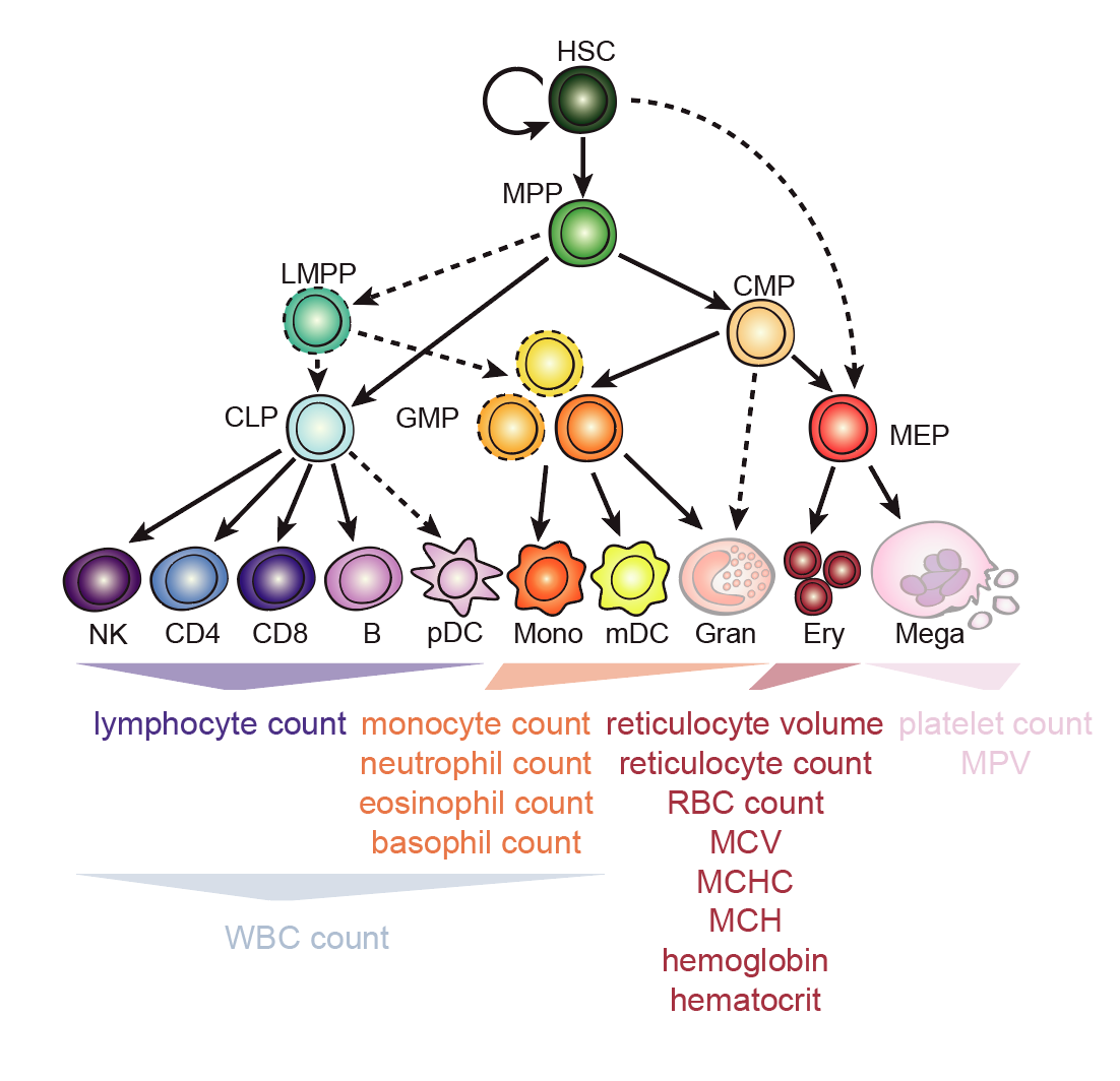
Figure 1. Overview of hematopoesis with cell types (top; note colors) and GWAS traits (bottom) explored thus far with gchromVAR.
Also, note that the traits are positioned under the hierarchy in accordance with our current understanding of where these cell traits manifest after differentiating. One might hypothesize that the terminal cell types may be the most enriched for those particular traits (e.g. erythroblasts should be enriched for GWAS signal for traits like red blood cell count). One may also expect late-stage progenitors (i.e. the cell types that occur before terminal differentation that may be multi-potent like CMPs or MEPs). With this in mind, we are ready to explore the gchromVAR results.
Building a RangedSummarizedExperiment
For using ATAC-seq or other chromatin accessibility data for gchromVAR, we recommend using the proatac pipeline to generate 1 set of consensus, equal-wdith peaks spanning the cellular phenotypes and synthesizing a singular counts table. These data for hematopoesis are already available in the extdata of gchromVAR. The format of the quantitative chromatin data for the key functionality is a RangedSummarizedExperiment, which we construct using the counts matrix and peak definitions. The last line of code also adds the GC content per peak, which is used in the background model.
countsFile <- paste0(system.file('extdata/paper',package='gchromVAR'), "/hemeCounts.tsv.gz")
peaksFile<- paste0(system.file('extdata/paper',package='gchromVAR'), "/hemePeaks.bed.gz")

peaksdf <- data.frame(fread(paste0("zcat < ", peaksFile)))
peaks <- makeGRangesFromDataFrame(peaksdf, seqnames = "V1", start.field = "V2", end.field = "V3")
counts <-  data.matrix(fread(paste0("zcat < ", countsFile)))
SE <- SummarizedExperiment(assays = list(counts = counts),
                               rowData = peaks,
                               colData = DataFrame(names = colnames(counts)))
SE <- addGCBias(SE, genome = BSgenome.Hsapiens.UCSC.hg19)
Importing GWAS summary statistics
Next, we want to overlap the GWAS summary statistics with our accessibility peaks. To facilitate this, we’ve created the importBedScore function, which will iteratively build another RangedSummarizedExperiment where the same peaks define the row space and the columns are defined as various GWAS annotations. The counts are quantitative measures of the total fine-mapped posterior probabilities of the variants overlapping those peaks.
files <- list.files(system.file('extdata/paper/PP001',package='gchromVAR'),
                    full.names = TRUE, pattern = "*.bed$")
head(read.table(files[1]))
## V1 V2 V3 V4 V5
## 1 chr1 25653526 25653527 region1 1.0000
## 2 chr1 24850597 24850598 region1 0.0242
## 3 chr1 24722451 24722452 region1 0.0103
## 4 chr1 24665802 24665803 region1 0.0096
## 5 chr1 24994340 24994341 region1 0.0096
## 6 chr1 25095653 25095654 region1 0.0061ukbb <- importBedScore(rowRanges(SE), files, colidx = 5)
str(ukbb)## Formal class 'RangedSummarizedExperiment' [package "SummarizedExperiment"] with 6 slots
## ..@ rowRanges :Formal class 'GRanges' [package "GenomicRanges"] with 6 slots
## .. .. ..@ seqnames :Formal class 'Rle' [package "S4Vectors"] with 4 slots
## .. .. .. .. ..@ values : Factor w/ 23 levels "chr1","chr2",..: 1 2 3 4 5 6 7 8 9 10 ...
## .. .. .. .. ..@ lengths : int [1:23] 39165 40692 33479 26870 27811 29215 26134 23199 18351 21123 ...
## .. .. .. .. ..@ elementMetadata: NULL
## .. .. .. .. ..@ metadata : list()
## .. .. ..@ ranges :Formal class 'IRanges' [package "IRanges"] with 6 slots
## .. .. .. .. ..@ start : int [1:451283] 10290 13252 16019 29020 96387 115440 237507 240798 521355 540679 ...
## .. .. .. .. ..@ width : int [1:451283] 501 501 501 501 501 501 501 501 501 501 ...
## .. .. .. .. ..@ NAMES : NULL
## .. .. .. .. ..@ elementType : chr "integer"
## .. .. .. .. ..@ elementMetadata: NULL
## .. .. .. .. ..@ metadata : list()
## .. .. ..@ strand :Formal class 'Rle' [package "S4Vectors"] with 4 slots
## .. .. .. .. ..@ values : Factor w/ 3 levels "+","-","*": 3
## .. .. .. .. ..@ lengths : int 451283
## .. .. .. .. ..@ elementMetadata: NULL
## .. .. .. .. ..@ metadata : list()
## .. .. ..@ elementMetadata:Formal class 'DataFrame' [package "S4Vectors"] with 6 slots
## .. .. .. .. ..@ rownames : NULL
## .. .. .. .. ..@ nrows : int 451283
## .. .. .. .. ..@ listData :List of 1
## .. .. .. .. .. ..$ bias: num [1:451283] 0.689 0.575 0.513 0.778 0.453 ...
## .. .. .. .. ..@ elementType : chr "ANY"
## .. .. .. .. ..@ elementMetadata: NULL
## .. .. .. .. ..@ metadata : list()
## .. .. ..@ seqinfo :Formal class 'Seqinfo' [package "GenomeInfoDb"] with 4 slots
## .. .. .. .. ..@ seqnames : chr [1:23] "chr1" "chr2" "chr3" "chr4" ...
## .. .. .. .. ..@ seqlengths : int [1:23] NA NA NA NA NA NA NA NA NA NA ...
## .. .. .. .. ..@ is_circular: logi [1:23] NA NA NA NA NA NA ...
## .. .. .. .. ..@ genome : chr [1:23] NA NA NA NA ...
## .. .. ..@ metadata : list()
## ..@ colData :Formal class 'DataFrame' [package "S4Vectors"] with 6 slots
## .. .. ..@ rownames : chr [1:16] "BASO_COUNT_PP001" "EO_COUNT_PP001" "HCT_PP001" "HGB_PP001" ...
## .. .. ..@ nrows : int 16
## .. .. ..@ listData :List of 1
## .. .. .. ..$ file: chr [1:16] "BASO_COUNT_PP001" "EO_COUNT_PP001" "HCT_PP001" "HGB_PP001" ...
## .. .. ..@ elementType : chr "ANY"
## .. .. ..@ elementMetadata: NULL
## .. .. ..@ metadata : list()
## ..@ assays :Reference class 'ShallowSimpleListAssays' [package "SummarizedExperiment"] with 1 field
## .. ..$ data: NULL
## .. ..and 14 methods.
## ..@ NAMES : NULL
## ..@ elementMetadata:Formal class 'DataFrame' [package "S4Vectors"] with 6 slots
## .. .. ..@ rownames : NULL
## .. .. ..@ nrows : int 451283
## .. .. ..@ listData : Named list()
## .. .. ..@ elementType : chr "ANY"
## .. .. ..@ elementMetadata: NULL
## .. .. ..@ metadata : list()
## ..@ metadata : list()With these two RSE objects created (SE for chromatin counts and ukbb for GWAS data), we can now run the core gchromVAR function, computeWeightedDeviations.
Computing weighted deviations
The functional execution having followed the previous steps is straight forward–
ukbb_wDEV <- computeWeightedDeviations(SE, ukbb)
zdf <- reshape2::melt(t(assays(ukbb_wDEV)[["z"]]))
zdf[,2] <- gsub("_PP001", "", zdf[,2])
colnames(zdf) <- c("ct", "tr", "Zscore")
head(zdf)
## ct tr Zscore
## 1 B BASO_COUNT 0.54028791
## 2 CD4 BASO_COUNT -0.08351059
## 3 CD8 BASO_COUNT -0.66325644
## 4 CLP BASO_COUNT 0.49815087
## 5 CMP BASO_COUNT 1.70456014
## 6 Ery BASO_COUNT -0.68111180The later steps just show re-formatted output for convenience. The last table, zdf provides a data frame of the Cell type (ct), trait (tr) and enrichment z-score for each of the 16x18 combinations.
Performing the lineage-specific enrichment test
A statistical way of determining how our results faired is to determine the relative positioning of lineage-specific enrichments. For each trait, we define the appropriate set of lineage-specific tissues (from Figure 1), and then annotate the results data frame. First, we define the four major lineages in hematopoesis:
Ery <- c("HSC", "MPP", "CMP", "MEP", "Ery")
Meg <- c("HSC", "MPP", "CMP", "MEP", "Mega")
Mye <- c("HSC", "MPP", "CMP", "LMPP", "GMP-A", "GMP-B", "GMP-C", "Mono", "mDC")
Lymph <- c("HSC", "MPP", "LMPP", "CLP", "NK", "pDC", "CD4", "CD8", "B")
Next, we annotate the data frame work lineage-specific (“LS”) enrichments:
zdf$LS  <-
    (zdf$tr == "BASO_COUNT" & zdf$ct %in% Mye) +
    (zdf$tr == "EO_COUNT" & zdf$ct %in% Mye) +
    (zdf$tr == "NEUTRO_COUNT" & zdf$ct %in% Mye) +
    (zdf$tr == "MONO_COUNT" & zdf$ct %in% Mye) +
    (zdf$tr == "WBC_COUNT" & zdf$ct %in% c(Mye, Lymph)) +
    (zdf$tr == "LYMPH_COUNT" & zdf$ct %in% Lymph) +
    (zdf$tr == "PLT_COUNT" & zdf$ct %in% Meg) +
    (zdf$tr == "MPV" & zdf$ct %in% Meg) +
    (zdf$tr == "MEAN_RETIC_VOL" & zdf$ct %in% Ery) +
    (zdf$tr == "HGB" & zdf$ct %in% Ery) +
    (zdf$tr == "HCT" & zdf$ct %in% Ery) +
    (zdf$tr == "MCH" & zdf$ct %in% Ery) +
    (zdf$tr == "MCV" & zdf$ct %in% Ery) +
    (zdf$tr == "MCHC" & zdf$ct %in% Ery) +
    (zdf$tr == "RBC_COUNT" & zdf$ct %in% Ery) +
    (zdf$tr == "RETIC_COUNT" & zdf$ct %in% Ery)
Finally, we can compute a Mann-Whitney Rank-sum statistic to determine the relative enrichment of the gchromVAR results compared to the non-lineage specific measures:
zdf$gchromVAR_pvalue <- pnorm(zdf$Zscore, lower.tail = FALSE)
gchromVAR_ranksum <- sum(1:dim(zdf)[1]*zdf[order(zdf$gchromVAR_pvalue, decreasing = FALSE), "LS"])
permuted <- sapply(1:10000, function(i) sum(1:dim(zdf)[1] * sample(zdf$LS, length(zdf$LS))))
pnorm((mean(permuted) - gchromVAR_ranksum)/sd(permuted), lower.tail = FALSE)
## [1] 5.075067e-15From this statistic, we can see that lineage-specific enrichments for much stronger for gchromVAR than we’d expect by chance. We quantified this for several related methods on the initial landing page, demonstrating the utility of our approach.
Extracting Individual Enrichments
Finally, we can do a simple Bonferonni-correction threshold to see that nearly all of the enrichments from gchromVAR are lineage specific. Moverover, these enrichments corroborate known biology in hematopoesis.
zdf[zdf$gchromVAR_pvalue < 0.05/288 , ]## ct tr Zscore LS gchromVAR_pvalue
## 74 CD4 LYMPH_COUNT 4.199441 1 1.337873e-05
## 75 CD8 LYMPH_COUNT 4.803311 1 7.803174e-07
## 95 CMP MCH 4.001357 1 3.149017e-05
## 96 Ery MCH 13.612421 1 1.689314e-42
## 104 MEP MCH 9.753007 1 8.954164e-23
## 114 Ery MCHC 7.839812 1 2.256098e-15
## 122 MEP MCHC 4.569496 1 2.444496e-06
## 132 Ery MCV 15.538675 1 9.493371e-55
## 140 MEP MCV 7.944465 1 9.751538e-16
## 150 Ery MEAN_RETIC_VOL 15.786382 1 1.930484e-56
## 158 MEP MEAN_RETIC_VOL 8.691358 1 1.790667e-18
## 169 GMP-A MONO_COUNT 5.206497 1 9.621961e-08
## 170 GMP-B MONO_COUNT 4.209538 1 1.279465e-05
## 177 Mono MONO_COUNT 4.755962 1 9.875178e-07
## 185 CMP MPV 3.753410 1 8.722274e-05
## 193 Mega MPV 5.750519 1 4.448507e-09
## 194 MEP MPV 4.013335 1 2.993347e-05
## 221 CMP PLT_COUNT 4.515496 1 3.158444e-06
## 222 Ery PLT_COUNT 4.606007 0 2.052373e-06
## 229 Mega PLT_COUNT 3.834510 1 6.290746e-05
## 230 MEP PLT_COUNT 4.981455 1 3.155391e-07
## 240 Ery RBC_COUNT 8.749975 1 1.066998e-18
## 248 MEP RBC_COUNT 6.477772 1 4.654340e-11
## 258 Ery RETIC_COUNT 8.634427 1 2.951099e-18
## 266 MEP RETIC_COUNT 4.256826 1 1.036750e-05